Getting Started: Defining an MCMC Algorithm

Overview

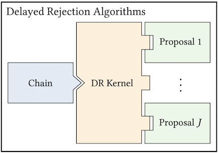
The goal of MCMC is to construct a Markov chain that is ergodic and has a given stationary distribution \(p(x)\). MUQ defines MCMC algorithms through three components: the chain, a transition kernel, and a proposal. This idea is illustrated below for Metropolis-Hastings and Delayed-Rejection algorithms.

In MUQ, the chain is the top level object in an MCMC definition. In particular, the SingleChainMCMC class is typically used to define a standard single-chain MCMC algorithm. The chain, of course, depends on the transition kernel. This corresponds to another abstract base class in the MUQ MCMC stack, the TransitionKernel class. The classic Metropolis-Hastings rule is implemented in the MHKernel class, but this is just one of many different transition kernels available in MUQ. Each of these kernels can be coupled with one of the proposal distributions implemented in MUQ. The proposal distributions are children of the abstract MCMCProposal base class.

Step 1: Defining the Problem

The first step in using MUQ's MCMC tools is to define the posterior distribution we want to sample. This is typically accomplished via the SamplingProblem class. The constructor of SamplingProblem takes a ModPiece that evaluates the log density \(\log p(x)\). It is also possible to pass another ModPiece that evaluates an additional quantity of interest that needs to be evaluated at samples of the target distribution.

Below is an example of defining a simple two dimensional Gaussian SamplingProblem.

The Gaussian class is used to define the target density. The Gaussian class can be used for either sampling or density evaluations. The AsDensity function returns a ModPiece that evaluates the log of the Gaussian density – exactly what the SamplingProblem needs.

C++

Python

Eigen::VectorXd mu(2);
mu << 1.0, 2.0;

Eigen::MatrixXd cov(2,2);
cov << 1.0, 0.8,
       0.8, 1.5;

auto targetDensity = std::make_shared<Gaussian>(mu, cov)->AsDensity();
auto problem = std::make_shared<SamplingProblem>(targetDensity);

mu = np.array([1.0,2.0])

cov = np.array([[1.0, 0.8],
                [0.8, 1.0]])

targetDensity = mm.Gaussian(mu,cov).AsDensity()
problem = ms.SamplingProblem(targetDensity)

Step 2: Assembling an Algorithm

Once the problem is defined, it's time to combine chain, kernel, and proposal components to define an MCMC algorithm. Below is an example combining the random walk MHProposal proposal with the usual Metropolis-Hastings MHKernel kernel in a single chain MCMC sampler. Note that additional options are specified in with boost::property_tree::ptree variables in c++ and dictionaries in python.

C++

Python

// Define the random walk proposal proposal
boost::property_tree::ptree propOpts;
propOpts.put("ProposalVariance", 1.0);
auto prop = std::make_shared<MHProposal>(propOpts, problem);

// Define the Metropolis-Hastings transition kernel
boost::property_tree::ptree kernOpts;
auto kern = std::make_shared<MHKernel>(kernOpts, problem, prop);

// Construct the MCMC sampler using this transition kernel
boost::property_tree::ptree chainOpts;
chainOpts.put("NumSamples", 2000);
chainOpts.put("BurnIn", 10);
chainOpts.put("PrintLevel", 3);

auto sampler = std::make_shared<SingleChainMCMC>(chainOpts, kern);

# Define the random walk proposal
propOpts = {"ProposalVariance" : 1.0}
prop = ms.MHProposal(propOpts, problem)

# Define the Metropolis-Hastings transition kernel
kernOpts = dict()
kern = ms.MHKernel(kernOpts, problem, prop)

# Construct the MCMC sampler
chainOpts = {'NumSamples': 2000,
             'BurnIn': 10,
             'PrintLevel' : 3}

sampler = ms.SingleChainMCMC(chainOpts, [kern])

Swapping Proposals

Individual components of the MCMC sampler can be changed without changing anything else. For example, the Metropolis-Adjusted Langevin Algorithm (MALA) uses the Metropolis-Hastings algorithm with a proposal that leverages gradient information to "shift" the random walk proposal towards higher density regions of \(p(x)\). Only the proposal distribution is different betweeen the MALA algorithm the basic standard Random Walk Metropolis (RWM) algorithm defined in the code above. Defining a MALA sampler in MUQ therefore only requires changing the proposal to use the MALAProposal class. This is shown below.

C++

Python

// Define the random walk proposal proposal
boost::property_tree::ptree propOpts;
propOpts.put("StepSize", 0.3);
auto prop = std::make_shared<MALAProposal>(propOpts, problem);

# Define the MALA proposal
propOpts = {"StepSize" : 0.3}
prop = ms.MALAProposal(propOpts, problem)

Changing Transition Kernels

Transition kernels are also interchangeable. Here is an example of constructing a delayed rejection sampler [Mira2001], where the first stage is a random walk proposal and the second stage uses a Langevin proposal.

C++

Python

// Define a list of proposals to use with the DR kernel
std::vector<std::shared_ptr<MCMCProposal>> props(2);

// Create the random walk proposal proposal
boost::property_tree::ptree propOpts;
propOpts.put("ProposalVariance", 1.0);
props.at(0) = std::make_shared<MHProposal>(propOpts, problem);

// Create the Langevin proposal
boost::property_tree::ptree malaOpts;
malaOpts.put("StepSize", 0.3);
props.at(1) = std::make_shared<MALAProposal>(malaOpts, problem);

// Define the delayed rejection kernel
boost::property_tree::ptree kernOpts;
auto kern = std::make_shared<DRKernel>(kernOpts, problem, props);

# Create the random walk proposal
rwmOpts = {"ProposalVariance" : 1.0}
rwmProp = ms.MHProposal(rwmOpts, problem)

# Create the Langevin proposal
malaOpts = {"StepSize" : 0.3}
malaProp = ms.MALAProposal(malaOpts, problem)

# Create the delayed rejection kernel
kernOpts = dict()
kern = ms.DRKernel(kernOpts, problem, [rwmProp, malaProp])

Step 3: Running the Sampler

We now have a sampling algorithm defined in the sampler variable in the code above, but no samples have been generated yet. To run the sampler and generate samples, we need to call the Run method, which accepts a starting point and returns the MCMC samples in the form of a SampleCollection.

C++

Python

// Define an initial state for the chain
Eigen::VectorXd x0(2);
x0 << 1.0, 2.0;

// Run the MCMC algorithm to generate samples. x0 is the starting location
std::shared_ptr<SampleCollection> samps = sampler->Run(x0);

# Define an initial state for the chain
x0 = np.array([1.0, 2.0])

# Run the MCMC algorithm to generate samples. x0 is the starting location
samps = sampler.Run([x0])

Step 4: Inspecting the Results

The Run function returns a SampleCollection object. SampleCollections store the state in the MCMC chain, weights for each state (in order to support importance sampling), as well as additional metadata that might have been stored for each sample by the MCMC components.

Here's an example of some basic things you might want to do with the sample collection.

C++

Python

// Return the number of samples in the collection
int numSamps = samps->size();

// Get various sample moments
Eigen::VectorXd mean = samps->Mean();
Eigen::VectorXd var = samps->Variance();
Eigen::MatrixXd cov = samps->Covariance();

// Create an Eigen matrix with all of the samples
Eigen::MatrixXd sampsAsMat = samps->AsMatrix();

// Extract metadata saved by the MCMC algorithm.
Eigen::MatrixXd logDensity = samps->GetMeta("LogTarget");
Eigen::MatrixXd gradLogDensity = samps->GetMeta("GradLogDensity_0"); // <- Only available when using gradient-based proposals (e.g., MALA)

# Return the number of samples in the collection
numSamps = samps.size()

# Get various sample moments
mean = samps.Mean()
var = samps.Variance()
cov = samps.Covariance()

# Create an Eigen matrix with all of the samples
sampsAsMat = samps.AsMatrix()

# Extract metadata saved by the MCMC algorithm.
logDensity = samps.GetMeta("LogTarget")
gradLogDensity = samps.GetMeta("GradLogDensity_0") # <- Only available when using gradient-based proposals (e.g., MALA)

Just like ModPieces can have multiple vector-valued inputs, the log density we're trying to sample might have multiple inputs, say \(p(x,y)\). In GetMeta("GradLogDensity_0"), the "_0" part of the string refers to index of the input that the gradient was taken with respect to, e.g., "_0" matches \(\nabla_x \log p(x,y)\) and "_1" would match \(\nabla_y \log p(x,y)\). More information on sampling problems with more than one input can be found in the Blocks and Kernel Composition section.

Assessing Convergence

The transition kernels used in MCMC methods guarantee that the target distribution \(p(x)\) is the unique stationary distribution of the chain. If the distribution of the initial state \(x^{(0)}\) is \(p(x)\), this stationarity property guarantees that all subsequent steps in the chain will also be distributed according to the target distribution \(p(x)\). In practice however, the reason we are using MCMC is because we can't generate samples of the target distribution and therefore can't guarantee \(x^{(0)}\sim p(x)\).

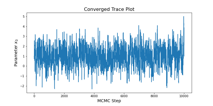
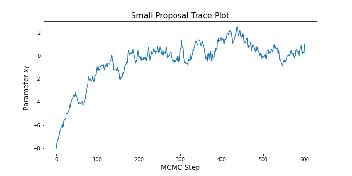
For an arbitrary starting point \(x^{(0)}\), we therefore need to assess whether the chain is long enough to ensure that the states have converged to the target distribution. Often the first step in assessing convergence is to look a trace plot of the chain. In python, we can convert extract a matrix of MCMC states from the SampleCollection class and then use matplotlib to create a trace plot (see below).

Python

sampMat = samps.AsMatrix()

plt.plot(sampMat[0,:])
plt.xlabel('MCMC Step',fontsize=14)
plt.ylabel('Parameter $x_0$',fontsize=14)
plt.title('Converged Trace Plot',fontsize=16)
plt.show()

For a sufficient long chain, this code might result in a trace plot like:

For a short chain that has not "forgotten" it's starting point, you might see a trace plot that looks like:

Trace plots are incredibly useful, but MUQ also has diagnostic tools for quantitatively assessing convergence using parallel chains and the \(\hat{R}\) diagnostic described in [Gelman2013], [Vehtari2021], and many other publications. The idea is to run multiple chains from different starting points and to assess whether the chains have reached the same distribution, presumably the target distribution \(p(x)\). Inter-chain means and variances are used to compute \(\hat{R}\) for each dimension of the chain. Values close to \(1\) indicate convergence. Here's an example running four chains and computing \(\hat{R}\) with MUQ:

C++

Python

unsigned int dim = 2;
unsigned int numChains = 4;
std::vector<std::shared_ptr<SampleCollection>> collections(numChains);

for(int i=0; i<numChains; ++i){
  Eigen::VectorXd startPt = RandomGenerator::GetNormal(dim);
  auto sampler = std::make_shared<SingleChainMCMC>(chainOpts, kern);
  collections.at(i) = sampler->Run(startPt);
}

Eigen::VectorXd rhat = Diagnostics::Rhat(collections);

dim = 2
numChains = 4
collections = [None]*numChains

for i in range(numChains):
    startPt = np.random.randn(dim);
    sampler = ms.SingleChainMCMC(chainOpts, [kern])
    collections[i] = sampler.Run([startPt])

rhat = ms.Diagnostics.Rhat(collections)

The Rhat function returns a vector containing the \(\hat{R}\) statistic for each component of the chain. Historically, values of \(\hat{R}<1.1\) have been used to indicate convergence. More recently however, it has been argued that this can sometimes lead to erroneous conclusions and a threshold of \(\hat{R}<1.01\) may be more appropriate. See [Vehtari2021] for more discussion on this point.

Measuring Efficiency

The \(\hat{R}\) statistic helps quantify if the MCMC sampler is indeed producing samples of the target distribution \(p(x)\). However, it does not indicate how efficiently the sampler is exploring \(p(x)\). This is commonly accomplished by looking at the effective sample size. MCMC produces a chain of correlated samples. Monte Carlo estimators using these correlated samples will therefore have a larger variance than an estimator using the same number of independent samples. The effective sample size (ESS) of a chain is the number of independent samples that would be needed to obtain the same estimator variance as the MCMC chain.

MUQ estimates the ESS of a single chain using the approach in [Wolff2004], which is based on the chain's autocorrelation function. The <SampleCollection> class has a ESS function that returns a vector of estimate ESS values for each component of the chain. Here's an example:

C++

Python

// Estimate the effective sample size
Eigen::VectorXd ess = samps->ESS();

// Estimate the Monte Carlo standard error (MCSE)
Eigen::VectorXd variance = samps->Variance();
Eigen::VectorXd mcse = (variance.array() / ess.array()).sqrt();

# Estimate the effective sample size
ess = samps.ESS()

# Estimate the Monte Carlo standard error (MCSE)
variance = samps.Variance()
mcse = np.sqrt(variance/ess)

Using Options Lists

The MCMC samplers defined above were created by programmtically creating a proposal, then a kernel, and then an instance of the SingleChainMCMC class. It is also possible to define MCMC algorithms entirely through string-valued options stored in either a boost::property_tree::ptree in c++ or a dictionary in python. MUQ internally registers each MCMC proposal and kernel class with a string. This allows scripts and executables to easily define difference algorithms entirely from text-based input files (e.g., JSON, YAML, XML). Below is code to recreate a random walk sampler using only the list of options.

C++

Python

JSON

C++ w/ JSON

Python w/ JSON

boost::property_tree::ptree options;

options.put("NumSamples", 10000); // number of MCMC steps
options.put("KernelList", "Kernel1"); // name of block that defines the transition kernel
options.put("Kernel1.Method", "MHKernel"); // name of the transition kernel class
options.put("Kernel1.Proposal", "MyProposal"); // name of block defining the proposal distribution
options.put("Kernel1.MyProposal.Method", "MHProposal"); // name of proposal class
options.put("Kernel1.MyProposal.ProposalVariance", 0.5); // variance of the isotropic MH proposal

auto mcmc = std::make_shared<SingleChainMCMC>(options,problem);

options = {
           "NumSamples": 10000, # number of MCMC steps
           "KernelList": "Kernel1",  # name of block that defines the transition kernel
           "Kernel1.Method": "MHKernel",  # name of the transition kernel class
           "Kernel1.Proposal": "MyProposal", # name of block defining the proposal distribution
           "Kernel1.MyProposal.Method": "MHProposal", # name of proposal class
           "Kernel1.MyProposal.ProposalVariance": 0.5 # variance of the isotropic MH proposal
         }

mcmc = ms.SingleChainMCMC(options,problem)

{
  "NumSamples" : 10000,
  "KernelList" : "Kernel1",
  "Kernel1" :
  {
    "Method" : "MHKernel",
    "Proposal" : "MyProposal",
    "MyProposal" :
    {
      "Method" : "MHProposal",
      "ProposalVariance" : 0.5
    }
  }
}

// Make Sure to include this at top of file
// #include <boost/property_tree/json_parser.hpp>

// Create an empty ptree
boost::property_tree::ptree options;

// Load the json contents into the ptree
boost::property_tree::read_json("mcmc-options.json", options);

auto mcmc = std::make_shared<SingleChainMCMC>(options,problem);

# Make sure to import json at start of script:
# import json

with open('mcmc-options.json','r') as fin:
  options = json.load(fin)

mcmc = ms.SingleChainMCMC(options,problem)

Blockwise Sampling and Kernel Composition

In the examples above, we considered sampling a density \(p(x)\) that had one vector-valued input \(x\). However, SamplingProblems can have more than one input. This situation commonly arises in hierarchical models, where we are interested in sampling a density \(p(x, \alpha)\) with additional vector-valued hyperparameters \(\alpha\) (e.g., the prior variance, or likelihood precision). Often it is more convenient, and sometimes more efficient, to sample \(x\) and \(\alpha\) one at a time. In the two-input case, the idea is to alternate through MCMC steps that first target the conditional \(p(x | \alpha^{(k)})\) for a fixed value \(\alpha^{(k)}\) and then target the conditional \(p(\alpha | x^{(k)})\). When variants of the Metropolis-Hastings rule are used for the MCMC transition kernel, this blockwise approach is known as Metropolis-in-Gibbs sampling.

MUQ defines Metrpolis-in-Gibbs samplers by passing in multiple transition kernels to the SingleChainMCMC class. For illustration, consider a simple target density \(p(x,y)=p(x)p(y)\), where \(x\) takes values in \(\mathbb{R}\), \(y\) takes values in \(\mathbb{R}^2\), \(p(x)=N(\mu_x,\sigma_x)\), and \(p(y)=N(\mu_y,\sigma_y)\). In MUQ, we could define this density using a WorkGraph as shown below

C++

Python

Eigen::VectorXd mux(1), varx(1);
mux << 1.0;
varx << 0.5;

auto px = std::make_shared<Gaussian>(mux,varx)->AsDensity();

Eigen::VectorXd muy(2), vary(2);
muy << -1.0, -1.0;
vary << 1.0, 2.0;

auto py = std::make_shared<Gaussian>(muy,vary)->AsDensity();

auto graph = std::make_shared<WorkGraph>();
graph->AddNode(px, "p(x)");
graph->AddNode(py, "p(y)");
graph->AddNode(std::make_shared<DensityProduct>(2), "p(x,y)");
graph->AddEdge("p(x)",0,"p(x,y)",0);
graph->AddEdge("p(y)",0,"p(x,y)",1);

auto pxy = graph->CreateModPiece("p(x,y)");

mux = np.array([1.0])
varx = np.array([0.5])

# Create the joint log density, which will have two inputs with sizes [1,2]
px = mm.Gaussian(mux,varx).AsDensity()

muy = np.array([-1.0,-1.0])
vary = np.array([1.0,2.0])

py = mm.Gaussian(muy,vary).AsDensity()

graph = mm.WorkGraph>()
graph.AddNode(px, "p(x)")
graph.AddNode(py, "p(y)")
graph.AddNode(mm.DensityProduct(2), "p(x,y)")
graph.AddEdge("p(x)",0,"p(x,y)",0)
graph.AddEdge("p(y)",0,"p(x,y)",1)

# Create the joint log density, which will have two inputs with sizes [1,2]
pxy = graph.CreateModPiece("p(x,y)")

In this example, the pxy variable is a two-input ModPiece that evaluates the log density \(\log p(x,y)\). The index of each input to this ModPiece can be specified through the BlockIndex option in the MCMCProposal class, which tells the proposal which input of the target density to target. The snippet below demonstrates this for two random walk proposals.

C++

Python

// Define the sampling problem as usual
auto problem = std::make_shared<SamplingProblem>(pxy);

// Construct two kernels: one for x and one for y
boost::property_tree::ptree opts;

// A vector to holding the two transition kernels
std::vector<std::shared_ptr<TransitionKernel>> kernels(2);

// Construct the kernel on x
opts.put("ProposalVariance", 3.0);
opts.put("BlockIndex", 0); // Specify that this proposal should target x
auto propx = std::make_shared<MHProposal>(opts, problem);
kernels.at(0) = std::make_shared<MHKernel>(opts, problem, propx);

// Construct the kernel on y
opts.put("ProposalVariance", 5.0);
opts.put("BlockIndex", 1); // Specify that this proposal should target y
auto propy = std::make_shared<MHProposal>(opts, problem);
kernels.at(1) = std::make_shared<MHKernel>(opts, problem, propy);

// Construct the MCMC sampler using this transition kernel
opts.put("NumSamples", 2000);
opts.put("BurnIn", 10);
opts.put("PrintLevel", 3);

auto sampler = std::make_shared<SingleChainMCMC>(chainOpts, kernels);

# Define the sampling problem as usual
problem = ms.SamplingProblem(pxy)

# Construct the proposal on x
opts = {
        "ProposalVariance": 3.0,
        "BlockIndex" : 0 # Specify that this proposal should target x
       }

propx = ms.MHProposal(opts, problem)

# Construct the proposal on y
opts = {
        "ProposalVariance": 5.0,
        "BlockIndex": 1
       }

propy = ms.MHProposal(opts, problem)

# Construct the MCMC sampler using this transition kernel
kernels = [ms.MHKernel({}, problem, propx),
           ms.MHKernel({}, problem, propy)]

sampler = SingleChainMCMC(opts, kernels)

See the pump test example for a more comprehensive example showing the use of Metropolis-in-Gibbs sampling for hyperparameters in a Gaussian likelihood function.