Individual ModPieces form the building blocks for larger more complicated models. MUQ makes it possible to connect ModPieces together on a computational graph to define larger models and enable the reuse of existing ModPiece implementations. The idea is to great graph of ModPieces where each node in the graph corresponds to a ModPiece and each edge represents a composition of one ModPiece with another. For example, if functions \(g(y)\) and \(f(x)\) are implemented as ModPieces, we can define the composition \(g(f(x))\) by creating a graph with two nodes and one edge from the output of \(f\) to the input of \(g\). Visually, the resulting graph would look something like

In MUQ, model graphs are defined using the WorkGraph class. The AddNode function in the WorkGraph class enables new model components to be added while the AddEdge allows us to make connections between the components. Here's an example of implementing the simple $g(f(x))$ model in MUQ. We use \(f(x)=\sin(x)\) and \(g(y)=\exp(y)\).
#include "MUQ/Modeling/WorkGraph.h"
#include "MUQ/Modeling/ModGraphPiece.h"
#include "MUQ/Modeling/CwiseOperators/CwiseUnaryOperator.h"

using namespace muq::Modeling;

int main(){
  unsigned int dim = 2;
  auto f = std::make_shared<SinOperator>(dim);
  auto g = std::make_shared<ExpOperator>(dim);

  auto graph = std::make_shared<WorkGraph>();

  graph->AddNode(f,"f");
  graph->AddNode(g,"g");
  graph->AddEdge("f",0,"g",0); // connect output 0 of f with input 0 of g

  auto gof = graph->CreateModPiece("f");

  return 0;
}The AddEdge function takes in the names of the nodes you wish to connect as well as integers specifying a particular output of f we want to connect to a particular input of g. In this case, both the SinOperator and ExpOperator ModPieces have a single input and a single input. Hence, we used "0" for both inputs and outputs. The CreateModPiece function returns a chile of the ModPiece class that uses the graph to evaluate \(f(g(x))\). Becuase it's a ModPiece, all of the usual ModPiece derivative functions are available. MUQ uses first and second order chain rules to analytically compute derivative information through the entire graph.
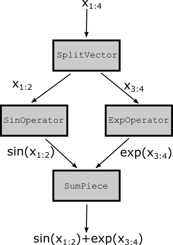
Consider another example where \(x\in\mathbb{R}^4\) and we want to implement a model that computes \(\sin(x_{1:2}) + \exp(x_{3:4})\). First, we'll use the SplitVector ModPiece to separate the vector \(x\) into two vectors: \(x_{1:2}\) and \(x_{3:4}\). After using the SinOperator and ExpOperator, we'll then sum the results using the SumPiece ModPiece. The resulting graph should look like

The code to construct this computational graph in MUQ is given below.
#include "MUQ/Modeling/WorkGraph.h"
#include "MUQ/Modeling/ModGraphPiece.h"
#include "MUQ/Modeling/SumPiece.h"
#include "MUQ/Modeling/SplitVector.h"
#include "MUQ/Modeling/CwiseOperators/CwiseUnaryOperator.h"

using namespace muq::Modeling;

int main(){
  auto f = std::make_shared<SinOperator>(2);
  auto g = std::make_shared<ExpOperator>(2);
  auto sum = std::make_shared<SumPiece>(2);

  // Will split x_{1:dim} into two equally sized vectors
  auto splitter = std::make_shared<SplitVector>(std::vector<int>{0,2}, // indices of output
                                                std::vector<int>{2,2}, // sizes of output
                                                4); // size of input

  auto graph = std::make_shared<WorkGraph>();

  graph->AddNode(splitter, "x12,x34");
  graph->AddNode(g,"g");
  graph->AddNode(f,"f");
  graph->AddEdge("x12,x34",0,"f",0); // connect output 0 of x12,x34 with input 0 of f
  graph->AddEdge("x12,x34",0,"g",0); // connect output 1 of x12,x34 with input 0 of g

  graph->AddNode(sum,"f+g");
  graph->AddEdge("f",0,"f+g",0); // connect output 0 of f with input 0 of f+g
  graph->AddEdge("g",0,"f+g",1); // connect output 0 of g with intpu 1 of f+g

  auto mod = graph->CreateModPiece("f+g");

  return 0;
}