Example
Basic Metropolis-in-Gibbs Sampling

Metropolis-in-Gibbs sampling of a simple hierarchical Bayesian model with Gaussian-Inverse Gamma target density.

Overview

The goal of this example is to demonstrate MCMC sampling with block updates. The problem is to sample a Gaussian distribution where the variance of the Gaussian is a random variable endowed with an inverse Gamma distribution. Thus, there are two "blocks" of interest: the Gaussian random variable and the variance hyperparameter. We will sample the joint distribution of both parameters by constructing a Metropolis-Within-Gibbs sampler.

Problem Formulation

Let $x$ denote the Gaussian random variable and $\sigma^2$ its variance, which follows an Inverse Gamma distribution. Notice that the joint density $\pi(x,\sigma)$ can be expanded in two ways: $$ \pi(x,\sigma^2) = \pi(x | \sigma^2)\pi(\sigma^2) $$ and $$ \pi(x,\sigma^2) = \pi(\sigma^2 | x)\pi(x). $$ We will use this to simplify the Metropolis-Hastings acceptance ratios below.

Now consider a two stage Metropolis-Hastings algorithm. In the first stage we take a step in $x$ with a fixed value of $\sigma^2$ and in the second stage we take a step in $\sigma^2$ with a fixed value of $x$. Using the Metropolis-Hastings rule for each stage, the algorithm is given by

1. Update $x$

   a. Propose a step in the $x$ block, $x^\prime \sim q(x | x^{(k-1)}, \sigma^{(k-1)})$

   b. Compute the acceptance probability using the expanded joint density $$\begin{eqnarray} \gamma &=& \frac{\pi(x^\prime | \sigma^{(k-1)})\pi(\sigma^{(k-1)})}{\pi(x^{(k-1)} | \sigma^{(k-1)}) \pi(\sigma^{(k-1)})} \frac{q(x^{(k-1)} | x^\prime, \sigma^{(k-1)})}{q(x^\prime | x^{(k-1)}, \sigma^{(k-1)})} \\ &=& \frac{\pi(x^\prime | \sigma^{(k-1)})}{\pi(x^{(k-1)} | \sigma^{(k-1)})} \frac{q(x^{(k-1)} | x^\prime, \sigma^{(k-1)})}{q(x^\prime | x^{(k-1)}, \sigma^{(k-1)})} \end{eqnarray}$$

   c. Take the step in the $x$ block: $x^{(k)} = x^\prime$ with probability $\min(1,\gamma)$, else $x^{(k)} = x^{(k-1)}$

2. Update $\sigma^2$

   a. Propose a step in the $\sigma^2$ block, $\sigma^\prime \sim q(\sigma | x^{(k)}, \sigma^{(k-1)})$

   b. Compute the acceptance probability using the expanded joint density $$\begin{eqnarray} \gamma &=& \frac{\pi(\sigma^\prime | x^{(k)})\pi(x^{(k)})}{\pi(\sigma^{(k-1)} | x^{(k)}) \pi(x^{(k)})} \frac{q(\sigma^{(k-1)} | \sigma^\prime, x^{(k)})}{q(\sigma^\prime | \sigma^{(k-1)}, x^{(k)})}. \\ &=& \frac{\pi(\sigma^\prime | x^{(k)})}{\pi(\sigma^{(k-1)} | x^{(k)})} \frac{q(\sigma^{(k-1)} | \sigma^\prime, x^{(k)})}{q(\sigma^\prime | \sigma^{(k-1)}, x^{(k)})}. \end{eqnarray}$$

   c. Take the step in the $\sigma^2$ block: $\sigma^{(k)} = \sigma^\prime$ with probability $\min(1,\gamma)$, else $\sigma^{(k)} = \sigma^{(k-1)}$

The extra complexity of this two stage approach is warranted when one or both of the block proposals $q(\sigma^\prime | \sigma^{(k-1)}, x^{(k)})$ and $q(x^\prime | x^{(k-1)}, \sigma^{(k-1)})$ can be chosen to match the condtiional target densities $\pi(\sigma^\prime | x^{(k)})$ and $\pi(x^\prime | \sigma^{(k-1)})$. When $\pi(x | \sigma^2)$ is Gaussian and $\pi(\sigma^2)$ is Inverse Gamma, as is the case in this example, the conditional target distribution $\pi(\sigma^2 | x)$ can be sampled directly, allowing us to choose $q(\sigma^\prime | \sigma^{(k-1)}, x^{(k)}) = \pi(\sigma^\prime | x^{(k)})$. This guarantees an acceptance probability of one for the $\sigma^2$ update. Notice that in this example, $\pi(x^\prime | \sigma^{(k-1)})$ is Gaussian and could also be sampled directly. For illustrative purposes however, we will mix a random walk proposal on $x$ with an independent Inverse Gamma proposal on $\sigma^2$.

Implementation

To sample the Gaussian target, the code needs to do four things:

1. Define the joint Gaussian-Inverse Gamma target density with two inputs and set up a sampling problem.

2. Construct the blockwise Metropolis-Hastings algorithm with a mix of random walk and Inverse Gamma proposals.

3. Run the MCMC algorithm.

4. Analyze the results.

Include statements

#include "MUQ/Modeling/Distributions/Gaussian.h"
#include "MUQ/Modeling/Distributions/InverseGamma.h"
#include "MUQ/Modeling/Distributions/Density.h"
#include "MUQ/Modeling/Distributions/DensityProduct.h"

#include "MUQ/Modeling/LinearAlgebra/IdentityOperator.h"
#include "MUQ/Modeling/ReplicateOperator.h"
#include "MUQ/Modeling/WorkGraph.h"
#include "MUQ/Modeling/ModGraphPiece.h"

#include "MUQ/SamplingAlgorithms/SamplingProblem.h"
#include "MUQ/SamplingAlgorithms/SingleChainMCMC.h"
#include "MUQ/SamplingAlgorithms/MCMCFactory.h"

#include <boost/property_tree/ptree.hpp>

namespace pt = boost::property_tree;
using namespace muq::Modeling;
using namespace muq::SamplingAlgorithms;
using namespace muq::Utilities;


int main(){

1. Define the joint Gaussian-Inverse Gamma target density

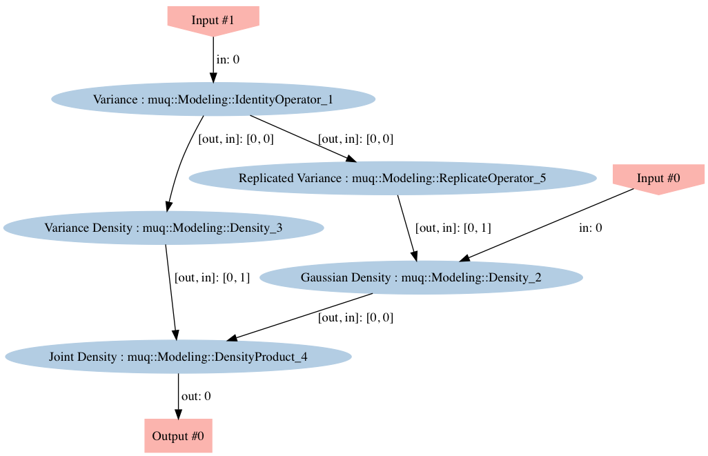
Here we need to construct the joint density $\pi(x | \sigma^2)\pi(\sigma^2)$. Combining models model components in MUQ is accomplished by creating a WorkGraph, adding components the graph as nodes, and then adding edges to connect the components and construct the more complicated model. Once constructed, our graph should look like:

Dashed nodes in the image correspond to model inputs and nodes with solid borders represent model components represented through a child of the ModPiece class. The following code creates each of the components and then adds them on to the graph. Notice that when the ModPiece's are added to the graph, a node name is specified. Later, we will use these names to identify structure in the graph that can be exploited to generate the Inverse Gamma proposal. Note that the node names used below correspond to the names used in the figure above.

  auto varPiece = std::make_shared<IdentityOperator>(1);

In previous examples, the only input to the Gaussian density was the parameter $x$ itself. Here however, the variance is also an input. The Gaussian class provides an enum for defining this type of extra input. Avaialable options are

• Gaussian::Mean The mean should be included as an input
• Gaussian::DiagCovariance The covariance diagonal is an input
• Gaussian::DiagPrecision The precision diagonal is an input
• Gaussian::FullCovariance The full covariance is an input (unraveled as a vector)

• Gaussian::FullPrecision The full precision is an input (unraveled as a vector)

  The | operator can be used to combine options. For example, if both the mean and diagonal covariance will be inputs, then we could pass Gaussian::Mean | Gaussian::DiagCovariance to the Gaussian constructor.

  In our case, only the diagonal covariance will be an input, so we can simply use Gaussian::DiagCovariance.

  Eigen::VectorXd mu(2);
  mu << 1.0, 2.0;

  auto gaussDens = std::make_shared<Gaussian>(mu, Gaussian::DiagCovariance)->AsDensity();

  std::cout << "Gaussian piece has " << gaussDens->inputSizes.size()
            << " inputs with sizes " << gaussDens->inputSizes.transpose() << std::endl;

Here we construct the Inverse Gamma distribution $\pi(\sigma^2)$

  const double alpha = 2.5;
  const double beta = 1.0;

  auto varDens = std::make_shared<InverseGamma>(alpha,beta)->AsDensity();

To define the product $\pi(x|\sigma^2)\pi(\sigma^2)$, we will use the DensityProduct class.

  auto prodDens = std::make_shared<DensityProduct>(2);

The Gaussian density used here is two dimensional with the same variance in each dimension. The Gaussian ModPiece thus requires a two dimensional vector to define the diagonal covariance. To support that, we need to replicate the 1D vector returned by the "varPiece" IdentityOperator. The ReplicateOperator class provides this functionality.

  auto replOp = std::make_shared<ReplicateOperator>(1,2);

  auto graph = std::make_shared<WorkGraph>();

  graph->AddNode(gaussDens, "Gaussian Density");
  graph->AddNode(varPiece, "Variance");
  graph->AddNode(varDens, "Variance Density");
  graph->AddNode(prodDens, "Joint Density");
  graph->AddNode(replOp, "Replicated Variance");

  graph->AddEdge("Variance", 0, "Replicated Variance", 0);
  graph->AddEdge("Replicated Variance", 0, "Gaussian Density", 1);
  graph->AddEdge("Variance", 0, "Variance Density", 0);

  graph->AddEdge("Gaussian Density", 0, "Joint Density", 0);
  graph->AddEdge("Variance Density", 0, "Joint Density", 1);

Visualize the graph

To check to make sure we constructed the graph correctly, we will employ the WorkGraph::Visualize function. This function generates an image in the folder where the executable was run. The result will look like the image below. Looking at this image closely, we see that, with the exception of the "Replicate Variance" node, the structure matches what we expect.

  graph->Visualize("DensityGraph.png");

Construct the joint density model and sampling problem

Here we wrap the graph into a single ModPiece that can be used to construct the sampling problem.

  auto jointDens = graph->CreateModPiece("Joint Density");

  auto problem = std::make_shared<SamplingProblem>(jointDens);

2. Construct the blockwise Metropolis-Hastings algorithm

The entire two-block MCMC algorithm described above can be specified using the same boost property tree approach used to specify a single chain algorithm. The only difference is the number of kernels specified in the "KernelList" ptree entry. Here, two other ptree blocks are specified "Kernel1" and "Kernel2".

"Kernel1" specifies the transition kernel used to update the Gaussian variable $x$. Here, it is the same random walk Metropolis (RWM) algorithm used in the first MCMC example.

"Kernel2" specifies the transition kernel used to udpate the variance $\sigma^2$. It could also employ a random walk proposal, but here we use to Inverse Gamma proposal, which requires knowledge about both $\pi(x | \sigma^2)$ and $\pi(\sigma^2)$. To pass this information to the proposal, we specify which nodes in the WorkGraph correspond to the Gaussian and Inverse Gamma densities.

  pt::ptree pt;
  pt.put("NumSamples", 1e5); // number of MCMC steps
  pt.put("BurnIn", 1e4);
  pt.put("PrintLevel",3);
  pt.put("KernelList", "Kernel1,Kernel2"); // Name of block that defines the transition kernel

  pt.put("Kernel1.Method","MHKernel");  // Name of the transition kernel class
  pt.put("Kernel1.Proposal", "MyProposal"); // Name of block defining the proposal distribution
  pt.put("Kernel1.MyProposal.Method", "CrankNicolsonProposal"); // Name of proposal class
  pt.put("Kernel1.MyProposal.ProposalVariance", 0.5); // Variance of the isotropic MH proposal
  pt.put("Kernel1.MyProposal.Beta", 0.25); // Variance of the isotropic MH proposal
  pt.put("Kernel1.MyProposal.PriorNode", "Gaussian Density");

  pt.put("Kernel2.Method","MHKernel");  // Name of the transition kernel class
  pt.put("Kernel2.Proposal", "GammaProposal"); // Name of block defining the proposal distribution

  pt.put("Kernel2.GammaProposal.Method", "InverseGammaProposal");
  pt.put("Kernel2.GammaProposal.InverseGammaNode", "Variance Density");
  pt.put("Kernel2.GammaProposal.GaussianNode", "Gaussian Density");

Once the algorithm parameters are specified, we can pass them to the CreateSingleChain function of the MCMCFactory class to create an instance of the MCMC algorithm we defined in the property tree.

  auto mcmc = MCMCFactory::CreateSingleChain(pt, problem);

3. Run the MCMC algorithm

We are now ready to run the MCMC algorithm. Here we start the chain at the target densities mean. The resulting samples are returned in an instance of the SampleCollection class, which internally holds the steps in the MCMC chain as a vector of weighted SamplingState's.

  std::vector<Eigen::VectorXd> startPt(2);
  startPt.at(0) = mu; // Start the Gaussian block at the mean
  startPt.at(1) = Eigen::VectorXd::Ones(1); // Set the starting value of the variance to 1

  std::shared_ptr<SampleCollection> samps = mcmc->Run(startPt);

4. Analyze the results

  Eigen::VectorXd sampMean = samps->Mean();
  std::cout << "Sample Mean = \n" << sampMean.transpose() << std::endl;

  Eigen::VectorXd sampVar = samps->Variance();
  std::cout << "\nSample Variance = \n" << sampVar.transpose() << std::endl;

  Eigen::MatrixXd sampCov = samps->Covariance();
  std::cout << "\nSample Covariance = \n" << sampCov << std::endl;

  Eigen::VectorXd sampMom3 = samps->CentralMoment(3);
  std::cout << "\nSample Third Moment = \n" << sampMom3 << std::endl << std::endl;

  return 0;
}

Complete Code

#include "MUQ/Modeling/Distributions/Gaussian.h"
#include "MUQ/Modeling/Distributions/InverseGamma.h"
#include "MUQ/Modeling/Distributions/Density.h"
#include "MUQ/Modeling/Distributions/DensityProduct.h"

#include "MUQ/Modeling/LinearAlgebra/IdentityOperator.h"
#include "MUQ/Modeling/ReplicateOperator.h"
#include "MUQ/Modeling/WorkGraph.h"
#include "MUQ/Modeling/ModGraphPiece.h"

#include "MUQ/SamplingAlgorithms/SamplingProblem.h"
#include "MUQ/SamplingAlgorithms/SingleChainMCMC.h"
#include "MUQ/SamplingAlgorithms/MCMCFactory.h"

#include <boost/property_tree/ptree.hpp>

namespace pt = boost::property_tree;
using namespace muq::Modeling;
using namespace muq::SamplingAlgorithms;
using namespace muq::Utilities;


int main(){

  auto varPiece = std::make_shared<IdentityOperator>(1);

  Eigen::VectorXd mu(2);
  mu << 1.0, 2.0;

  auto gaussDens = std::make_shared<Gaussian>(mu, Gaussian::DiagCovariance)->AsDensity();

  std::cout << "Gaussian piece has " << gaussDens->inputSizes.size()
            << " inputs with sizes " << gaussDens->inputSizes.transpose() << std::endl;

  const double alpha = 2.5;
  const double beta = 1.0;

  auto varDens = std::make_shared<InverseGamma>(alpha,beta)->AsDensity();

  auto prodDens = std::make_shared<DensityProduct>(2);

  auto replOp = std::make_shared<ReplicateOperator>(1,2);

  auto graph = std::make_shared<WorkGraph>();

  graph->AddNode(gaussDens, "Gaussian Density");
  graph->AddNode(varPiece, "Variance");
  graph->AddNode(varDens, "Variance Density");
  graph->AddNode(prodDens, "Joint Density");
  graph->AddNode(replOp, "Replicated Variance");

  graph->AddEdge("Variance", 0, "Replicated Variance", 0);
  graph->AddEdge("Replicated Variance", 0, "Gaussian Density", 1);
  graph->AddEdge("Variance", 0, "Variance Density", 0);

  graph->AddEdge("Gaussian Density", 0, "Joint Density", 0);
  graph->AddEdge("Variance Density", 0, "Joint Density", 1);

  graph->Visualize("DensityGraph.png");
  auto jointDens = graph->CreateModPiece("Joint Density");

  auto problem = std::make_shared<SamplingProblem>(jointDens);

  pt::ptree pt;
  pt.put("NumSamples", 1e5); // number of MCMC steps
  pt.put("BurnIn", 1e4);
  pt.put("PrintLevel",3);
  pt.put("KernelList", "Kernel1,Kernel2"); // Name of block that defines the transition kernel

  pt.put("Kernel1.Method","MHKernel");  // Name of the transition kernel class
  pt.put("Kernel1.Proposal", "MyProposal"); // Name of block defining the proposal distribution
  pt.put("Kernel1.MyProposal.Method", "CrankNicolsonProposal"); // Name of proposal class
  pt.put("Kernel1.MyProposal.ProposalVariance", 0.5); // Variance of the isotropic MH proposal
  pt.put("Kernel1.MyProposal.Beta", 0.25); // Variance of the isotropic MH proposal
  pt.put("Kernel1.MyProposal.PriorNode", "Gaussian Density");

  pt.put("Kernel2.Method","MHKernel");  // Name of the transition kernel class
  pt.put("Kernel2.Proposal", "GammaProposal"); // Name of block defining the proposal distribution

  pt.put("Kernel2.GammaProposal.Method", "InverseGammaProposal");
  pt.put("Kernel2.GammaProposal.InverseGammaNode", "Variance Density");
  pt.put("Kernel2.GammaProposal.GaussianNode", "Gaussian Density");

  auto mcmc = MCMCFactory::CreateSingleChain(pt, problem);

  std::vector<Eigen::VectorXd> startPt(2);
  startPt.at(0) = mu; // Start the Gaussian block at the mean
  startPt.at(1) = Eigen::VectorXd::Ones(1); // Set the starting value of the variance to 1

  std::shared_ptr<SampleCollection> samps = mcmc->Run(startPt);

  Eigen::VectorXd sampMean = samps->Mean();
  std::cout << "Sample Mean = \n" << sampMean.transpose() << std::endl;

  Eigen::VectorXd sampVar = samps->Variance();
  std::cout << "\nSample Variance = \n" << sampVar.transpose() << std::endl;

  Eigen::MatrixXd sampCov = samps->Covariance();
  std::cout << "\nSample Covariance = \n" << sampCov << std::endl;

  Eigen::VectorXd sampMom3 = samps->CentralMoment(3);
  std::cout << "\nSample Third Moment = \n" << sampMom3 << std::endl << std::endl;

  return 0;
}